
A thesis submitted to the faculty of the University of Utah in partial fulfillment of the requirements for the degree of Doctor of Philosophy
I express my appreciation to Dr. David C. Evans, Dr. Ivan E. Sutherland, and Dr. Dan Cohen for their great insight, help, and encouragement in the development of this work. The many hours they have spent with me in discussion have provided the intellectual stimulus required to carry on this research.
I am deeply indebted to Dr. Thomas G. Stockham, whose encouragement and friendship made this document possible. Without the time and effort given unselfishly by Dr. Stockham, this document would not exist.
Many thanks to Dr. William M. Newman whose suggestions concerning the manuscript were invaluable.
Thanks also to Linda Rae Buys for her help in typing the manuscript.
Lastly, I would like to thank my wife, Marva, for her unselfish love and help. Without her understanding and kindness, this research would not have been possible.
The application of computer graphics to problem solving has increased over the past few years. The representation of data in the form of line drawings, graphs, charts, diagrams and line plots has been explored extensively. This paper addresses itself to some new techniques used to solve problems associated with extending the power of computer graphics to include black and white, and color shading. In particular it presents a new method for converting data describing three-dimensional objects into data that can be used to generate two-dimensional halftone images. It deals with some problems that arise in black and white, and color shading.
The past few years have seen an enormous increase in the use of computer graphics. Nevertheless, the medium is still very restricted and primitive. [5] Present day equipment makes it impossible to achieve the pictorial realism that a graphic artist can attain. Coloring, shading, texture, and lighting effects are not available to the computer graphics user. With the present state of computer graphics in mind it is meaningful to ask what current technology can do to enhance the power of computer graphics. The aspects we would like to control may include intensity, color, and location of light sources; reflectance, surface texture, and coloring of the objects; and general illumination and atmospheric interference in the picture field. If these parameters can be controlled then computer graphics will offer a powerful tool for generating visual images.
This paper will address itself to some of the problems that arise in trying to attain the above goals. In particular it will deal with the problem of converting data that describes objects in three-dimensional space into data that can generate a two-dimensional picture representation of those objects. This problem is generally called the Hidden Line or Hidden Surface problem. The final section of this paper discusses the illumination, coloring and shading of picture representations of three-dimensional objects, and the display file structures that generate raster scan images on a display.
The description of the philosophy is best given by describing the motivation behind it. Suppose I examine a picture of a table with pencils on it. I quickly determine that large areas on top of the table are open and therefore have little information content. I scan over these areas searching out complex features such as a pencil. I dwell on a complex portion until I assimilate the information associated with it. From there I scan to other areas of the picture looking for additional complexity. In scanning the picture in this way I seem to spend little or no time on simple areas. Complex areas seem to present themselves to me as subproblems requiring a solution. I seem to reduce these problems into further subproblems until I either solve the subproblem or don't care anymore.
New algorithms for removing hidden surfaces which emulate the above process will now be discussed. Consider the view plane as a square picture. Either its contents are simple enough to process with some decision procedure or they are not sufficiently simple. If they are not, then we subdivide the square into four subsquares and ask the same question about the contents of the first subsquare as was asked about the parent square. This process is repeated recursively until one of two conditions holds with respect to a subsquare. If the contents of the square are simple enough to process, then data is put into a display file. If the square is as small or smaller than the desired resolution of the picture, then put a reference to the surface nearest to the observer into the display file.
The decision procedure that determines if subdivision of squares is necessary can be simple. Suppose a picture is of a set of planar polygons. We will generally subdivide a square unless one of two conditions holds. The projections of the polygons onto the view plane do not intersect with the square; or the square is surrounded by a projected polygon which is in front of other extended polygons within the square. Figure 1a illustrates what a view plane may look like if subdivided by the above process.

This criteria for subdivision will find all resolution size squares along the visible edges and all resolution size squares along the visible intersections of planes. This is exactly what we want. It locates all the points along the visible edges and intersections of the objects.
The process of subdividing the picture can be thought of as a logarithmic search for points where there is a change in the characteristics of the picture. The process can also be thought of as a scheme for finding locally simple geometric phenomena in portions of the view plane. Some observers characterize the algorithm as being what Floyd [3] calls non-deterministic. Another point of view sees the algorithm as making a tree of goals. As a goal is considered, a decision is made about its difficulty. If it cannot be achieved with the methods at hand, the algorithm generates subgoals (four). The first subgoal is now considered. This process is repeated recursively until either success is reported at some subgoal or until success is reported by default (In our case when the resolution of the picture is reached). When success is reported, the next subgoal at the same level (the brother) is considered. If all subgoals of a given goal have reported success, then the goal itself reports success. This order of examining goals and their subgoals is called a prefix ordering of the tree. In any event the important thing is that a difficult problem can successfully be divided into smaller, easier subproblems. This approach has many programming and data structuring advantages.
Subdividing the picture in a prefix order allows the computing associated with each square to be reduced by saving information about what happened in the larger parent squares. It is useful to save information invariant under the operation of subdivision. Such information can be called inherited. Taking advantage of inherited information can significantly reduce the computation associated with small squares.
Let us consider how inherited information might be used when a square and a polygon are disjoint. In this case the fact that the polygon and square are disjoint is inherited by all subsquares of that square, i.e., the subsquares are also disjoint with the polygon. When inherited information given in this example is used, it is generally true that the number of planar polygons processed becomes smaller as the squares examined get smaller. Using this fact allows large amounts of data not relevant to the local problems to be shelved. Saving the level of refinement at which the data is shelved allows the reconsideration of that data when coming up out of the subdivision process. Data is reintroduced at the level at which it was shelved so that brother squares at that level may be correctly processed.
The decision procedure that determines if a square is to be subdivided is important, If the procedure is relatively simple, then many subsquares may be processed. If the procedure is complex, then a fewer squares may be processed and yet computation per square may be high. In our discussion of the hidden surface algorithm three decision procedures will be discussed. The first will be discussed now. The last two will be introduced under the heading Variations on the Theme. Let us assume that the input to the algorithm is any collection of planar polygons in three-space. Also assume that a polygon k is given as a sequence
{Pki = (Xki, Yki, Zki), i=1, 2, ...n}
of n ordered planar points that form a directed closed path in three-space. Let σ be a map from three-space onto the view plane P such that
(Pki σ = (P'ki), for all i. Let dk(u,v,w) be equal to the distance from the point (u,v,w) on the view plane to the point (x,y,z) on the plane of polygon k such that (x,y,z) σ = (u,v,w), (see Figure 2). We can now describe a compact decision procedure that will remove hidden surfaces from the representation on P.

There are three basic relationships that have to be established between each polygon and the square being processed.
(see Figures 3a, 3b, and 3c). Note that condition 1 and 2 may not be mutually exclusive (see Figure 3d).
To determine which of these relationships exists, tests are made on the vertices of the polygon to determine if any are in the square. If any vertex of the polygon is in the square, then condition 2 is true. The edges that comprise each polygon are then individually checked to see if any intersect the square. This is done by seeing if either of the segments that are the diagonals of the square intersect the given edge. If any edges lie within the square then although condition 1 might be true we will assume condition 2 is true, e.g. Figure 3d. If no vertices or edges are within the square, then one corner (wj, uj, Vj) of the square is checked to see if it is in the interior of the polygon. This is done by letting R be any ray in the view plane P eminating from (wj, uj, vj). Now each edge of the polygon is checked against R to see if it crosses R. Also the direction in which edges cross is recorded. If the number of positive crossings equals the number of negative crossings, then the square is on the exterior of the polygon, (condition 3) otherwise, it is wholly inside (condition 1).


Once the relationships between the square and the polygons have been determined, subdivision of the square will occur unless one of the following conditions is satisfied, Is there a polygon satisfying condition 1 that hides all other polygons? More precisely, does there exist a polygon m satisfying condition 1 such that dm (uj, vj, wj) = min {di(uj, vj, wj) ] for all i ≠ m such that polygon i satisfies condition 1 or 2} for j=1,2,3,4 where (uj, vj, wj) are the corners of the square? If such a polygon exists, then subdivision does not occur. The other condition, where subdivision does not occur, is satisfied provided all polygons have condition 3 with the square, i.e., the square sees nothing.
Fortunately, in practice, we are able to simplify the tests for the relationships between polygons and squares. Let the view plane P be the X,Y plane and the projection be an orthogonal projection onto that plane. This assumption is not restrictive if the polygons are put through appropriate translation, rotation, clipping, and perspective transformations before projection. If the above special case is assumed, then P'ki= (Xki, Yki, Zki, 0) and dk(x,y,0)=Ax+By+C where Z= Ax+By+C is the transformed plane of the polygon in question, Also if the ray used in checking for condition 1 is assumed to have zero slope, then computation is simplified.
The decision procedure just described will produce resolution size squares along visible edges and intersection of the polygons. If these are directly displayed then a line drawing of the object with hidden surfaces removed will result, See Figure 5a
.The preceding discussion has mentioned nothing about the data structures that are used in implementing the algorithm. We assume that the input to the algorithm is restricted to be a set of arbitrary planar polygons in three-space.
Polygons can be input in a variety of ways. They can be considered to be a sequence of points (xi, yi, zi) in three-space that form a closed path. They can be considered to be an initial point (X0,Y0,Z0) followed by increments (ΔXi,ΔYi,ΔZi) from the previous point to form a closed path. A third way to specify the polygons given to the algorithm is to give the x and y coordinates of the points defining the polygons plus the equations of the planes of the polygons in the form Ax + By + Cz + D = 0. Any of these input schemes or other more elaborate schemes are useful depending on the application.
Along with the points that make up the polygons the number and order of points in each polygon is important in the input. Other data relevant to the polygons are an array of pointers making the set of input polygons into a list. This list structure is important in dealing with the inherited information discussed earlier.
Another essential data structure is that which is output during execution of the algorithm. I call this the display file. The nature of the display file is determined by the decision procedure used to decide if subdivision of a square is necessary. If the decision procedure is the one described earlier, then the display file consists of the points (x,y) on the view plane that are either on visible boundaries of polygons or on visible intersections of polygons. Information associated with these points in the display file depends on the type of picture and shading to be produced. The choice of a particular decision procedure is influenced by the capability of the display processor. Let us now explore these data structures in the context of the algorithm.
The list structure that we impose on the set of input polygons facilitates the exploitation of the inherited properties of the squares. For instance, the relationship between a given square and polygon can be one of three types. The square is wholly contained within the polygon. The square can contain an edge or vertex of the polygon. Or the square and polygon can be disjoint. The first and third of these conditions are inherited by all subsquares of a square. Suppose we treat the set of polygons as a list broken into three parts. The first part is all those polygons satsifying condition 1, the second part those satisfying condition 2, and the third those satisfying condition 3. Make the pointer to the first of the list of polygons point to the head of part 1. All polygons in part 1 surround any subsquare and therefore need not be checked for this condition. If a polygon in part 2 is found, upon checking, to surround the current subsquare, then this polygon can be inserted on the tail of part 1 for use in the next level of recursion. If any polygon in part 2 is found to be disjoint with the current subsquare, then this polygon can be inserted at the head of part 3 for use in the next level of recursion. Polygons in part 3 need not be examined at all. Conditions 1 and 3 are inherited by all subsquares of a given square. Condition 2 may not be. For this reason each polygon satisfying condition 2 must be checked with respect to each subsquare to see which of the three conditions holds. If we keep pointers to the end of part 1 and to the beginning of part 3 for each level in the recursion, then given any level we can determine what relationships the polygons have with the current square at that level. See Figure 4b for an example of a recursion and the list associated with it.


The list described above nicely structures some of the inherited information. Other information that is inherited by the squares is not easily handled by the list. An example of this occurs when a polygon has exactly one edge that intersects the square. Note that if this is the case then only one edge need be checked for intersection with any subsquares. This type of inherited information can be saved by tagging each polygon with the level at which the condition was first discovered plus the number of the edge that crosses the square. Other inherited information can be utilized when a polygon surrounding the current square is in front of other polygons. The polygons that are hidden in this way need not be examined in any subsquares. These polygons are flagged in a way similar to the one above. By saving more information with each polygon, time could conceivably be saved but storage costs may be high, For this reason additional information with each polygon has not been saved but instead has been recomputed when needed.
It is pertinent at this time to explore what might be done to reduce the number of output squares. This question is related to the decision procedure that decides if a square is too complicated to handle and therefore must be subdivided.
One approach taken to cut down the number of output squares is to terminate the subdivision of squares whenever at most one line of a polygon or intersection of two polygons is contained in the square. If this decision procedure is used, then an example of the resulting mosaic of squares is given in Figure 1b. We can see from comparing Figure 1a and Figure 1b that this technique reduces the number of squares that need be examined in the algorithm. Since the additional logic required in the decision procedure is not excessive, the adoption of this procedure may result in faster execution.
Another approach that can be used to implement the general philosophy of the hidden surface algorithm dictates that squares may not be the most desirable geometric entity to subdivide. This approach might suggest that since scan lines are the ultimate output, scan lines should be the construct to be subdivided. Although there are no conceptual advantages to this method, data structuring and memory management schemes can be invoked that may produce savings.
The basic strategy of this approach assumes, as in the previous cases, that a collection of planar polygons are input to the algorithm. If a list is associated with the array of points of the polygons, then this list can reflect the order of the points such that they coordinate of the points decreases as the list is followed. This implicit sorting of the points allows the edges of the polygons to be entered and deleted from a current edge list as they are germane to the computation of successive scan lines. An edge enters the list when the y coordinate of the scan line matches the greater of the y coordinates of the edge. The edge is deleted when the other y coordinate is matched by the y coordinate of the scan line. When an edge is introduced into the list several facts are stored with it. The polygon to which the edge belongs is stored. The initial x coordinate of the edge along with the change in x with respect to y is stored.
Under this approach the strategy for processing a given scan line coincides with the strategy for the entire picture in the previously described schemes. The scan line is recursively divided in half if its contents are too complicated to process. This technique of implementation allows the inherited information to be utilized to its full extent and also allows for a much simpler computation on the relationship between a segment of a scan line and a polygon. This method has the disadvantage, however, that it must go through the subdivision process for each scan line that intersects some polygon.
Up until now we have discussed three variations for the implementation of the hidden surface algorithm. The strategy that minimizes time in the context of the algorithm's philosophy can only be obtained by examining computation trade-offs within the algorithm. This paper will not dwell on these problems since the evidence we have collected does not conclusively indicate that one method is superior to another.
There is something common to all types of display files the algorithms may output. The information in the display file represents the visible geometric aspects of the picture. The way the file represents the visible geometry is a function of the decision procedure that allows the subdivision of squares. If the subdivision of a square continues when any visible boundaries are in the square, then the display file consists of the points along the visible boundaries and intersection of the polygons. In this case the display file is a set of points (x,y). If line representations of the picture are desired, then the action to be taken is quite simple. The set of (x,y) points must be sorted into the order that corresponds to the way the raster sweeps the display, i.e., if the raster sweeps left to right, top to bottom, then sort the points x ascending within y descending. If the scan proceeds and each point in the scan is compared with the first point in the sorted display file until a match is found, then that point can be intensified. The scan can now be continued until a match with the next point in the display file is found. This process of matching and advancing the scan and display file is continued until the entire picture is produced (see Figure 5a). The above scheme is basically the same for all of the techniques that we have developed for converting the geometry of a picture into a raster scan image. In all these techniques the display file is sorted so that its elements are encountered in the same order as the raster sweeps the screen. If the geometry consists of points as in the above case, then the points are encountered in the same order as the scan sweeps those points. If the geometry consists of line segments as is the case if the second decision procedure is adopted, then line segments are ordered so they are encountered sequentially by the raster.
To build a picture from line segments the approach taken is more complicated. Once a line is encountered by the raster it is used in generating the picture until the line segment is exhausted by the scanning process. Memory is dedicated for storing the line segments that are currently pertinent to the generation of the display. When these line segments are encountered as the scan sweeps the display, they are inserted into memory. The segments are then generated from memory point by point until exhausted. They are then deleted. Since the algorithm cannot allow line segments to intersect, it is seen that the updating of the segment from scan line to scan line can never alter their order in the memory for current lines. For this reason the memory in which the segments are stored can be thought of as a circular queue. In conjunction with the processing of segments, new segments are introduced into the queue as they are encountered by the raster. Information that is required with each line segment varies with the kind of shading desired. If one wants to display the lines themselves, then the following is needed: The initial point of each segment (x0, y0), the inverse of the slope Δx/Δy and the last y coordinate of the segment yL. The segment is introduced into the memory based on x0 and y0. It is deleted when a match on yL occurs. The intermediate values are attained by updating x0 with Δx/Δy. This scheme requires no searching and therefore is quite efficient.
If halftone shading of the polygons is desired with the first kind of display file, then the action to be taken is simple. When the polygons are passed to the hidden line routine, a shading function is computed for each polygon. This function is in terms of x and y and yields a brightness level for that polygon at a point (x,y). In the process of hidden line removal each display file entry (x,y) is tagged with a pointer to the polygon seen immediately to its right. If there is no polygon to the right then a null polygon is used. With this display file it is easy to produce a shaded picture. The display file is sorted x ascending within y descending. As each point is encountered by the scan, the shading function associated with the polygon is put into effect along the scan line until the next point is encountered by the scan and its shading function takes effect. This method allows a flexible use of the halftone display. By overlaying three shading functions corresponding to the additive primary color components on a given polygon it is quite easy to achieve full color capabilities in the shading of the objects displayed. What these shading functions are and how they are achieved will be the next topic of discussion.
The production of shaded pictures in black and white or natural color presents some very unusual problems. The variables of which the worker must be aware in the consideration of a model include the following:
In lieu of building a mathematical color model that will compensate and account for all of the above variables, a description will be given of color and shading models that will yield acceptable results These models have been constructed on empirical considerations and should in no way be regarded as models for colorimetry, optics, or psychophysics. The shading models and color models that have been used will be discussed in the order in which they evolved.
The simplest approach to black and white shading is to ignore all aspects of lighting except the angle between a ray from the light source and the normal to the polygon under consideration. If this is done then the shade of a polygon can be given by s= K |cos θ| + M here K and M adjust the magnitude of the numbers going to the display. θ is the angle between a ray from the source and the normal to the polygon. This shading rule produces acceptable real-looking results in most cases. Its drawback can be noticed when a picture of two overlapping separated parallel planes is made and the edge that overlaps cannot be detected.
The second type of shading model considers the shading of a point on a polygon to be a function of its distance from the light source. The function can be given by s= (K |cos θ|) / (r + C) + M. Here r is the distance of the point from the light source. K, C, and M should be adjusted to the values of r so that an acceptable range of numbers is fed to the display.
It may be said at this point that illumination decreases with r2 instead of r, and therefore r2 should be used. Practically speaking the only reason that distance is considered at all is to eliminate the problem of the parallel planes described in the previous scheme. The use of r2 can change the light intensity so radically over a short distance that the resulting pictures look unnatural. In fact, depending on the values of r, the use of sqrt(r) may produce better results than r. In any event, the second scheme of shading produces good black and white pictures (see Figure 5b).
To open the discussion about producing color, a straightforward extension of the above will be considered. For each of the additive primary colors (red, green, and blue) a shading will be given. [2] They are:
sR = (R |cos θ|) / (r + C) + M
sG = (G |cos θ|) / (r + C) + M
sB = (B |cos θ|) / (r + C) + M
Here sR, sG and sB, are the shading functions for the red, green, and blue color components of the polygon. The values of R, G, and B define the color of the polygon. What this means will now be explained.
The aspects of color include hue, intensity, and saturation. By setting the values of R, G, and B the three aspects of color may be specified.
The saturation of a color, in a sense, refers to the purity of the color. Pastel colors are unsaturated, brilliant colors are more saturated. The control of saturation with the formulas consists in adding or subtracting a constant to or from each of the three values R, G, and B.
Adding a constant reduces saturation of the color. Subtracting a constant increases saturation. The maximum saturation under these circumstances occurs when one or more of R, G, and B has the value zero.
Hue is the aspect of color that is most often associated with the word color. When one or more of R, G, and B are zero, then hue is determined by the proportions of remaining values. If red and green are mixed additively then yellow results, If blue and green are mixed then cyan (sky blue) results, If red and blue are mixed then magenta (lavender) results. Variations in the ratios of these mixtures result in variations in hue.
This paper has dealt with some of the basic problems that arise in producing two-dimensional halftone images of objects described in three-space. Some new attitudes and techniques have been discussed. With these attitudes and techniques as a basis, it is natural to ask: What extensions to this kind of graphics are possible? Following is a list of potential extensions: The extension of the input to include curved surfaces as well as planar polygons; the inclusion of lines and text in the same image as halftone shading; the ability to specify transparency and translucency of objects as well as reflectivity; the ability to specify multiple light sources of various locations, intensities and colors; the ability to specify the filtering qualities of an atmosphere in order to simulate fog and haze. Each of these topics provide a research area in which no extensive work has been done.
I feel strongly that this enhancement of visual communication between machine and man will yield great advances in the effective utilization of computers. Data which once was represented as a sea of printed numbers can be represented as revealing visual patterns. Highly complex abstract relationships can be understood at a glance by their reduction to visual relationships. (See Figure 6) The development and perfection of this computation tool will allow man to more easily and effectively understand and solve the problems that confront him.

These figures are representative of various kinds of shading rules. (a) displays only those points in the display file. This method yields a line drawing. (b) uses the display file along with shading functions associated with each polygon. (c) is a color representation that uses shading functions associated with each additive primary color. There are no specular components in this picture. (d) is the same as (c) except that specular components have been added to increase realism.
The computation time required between the input of the 654 polygons of the above picture and the final construction of the display file is about one minute on a Univac 1108 using a Fortran V program.
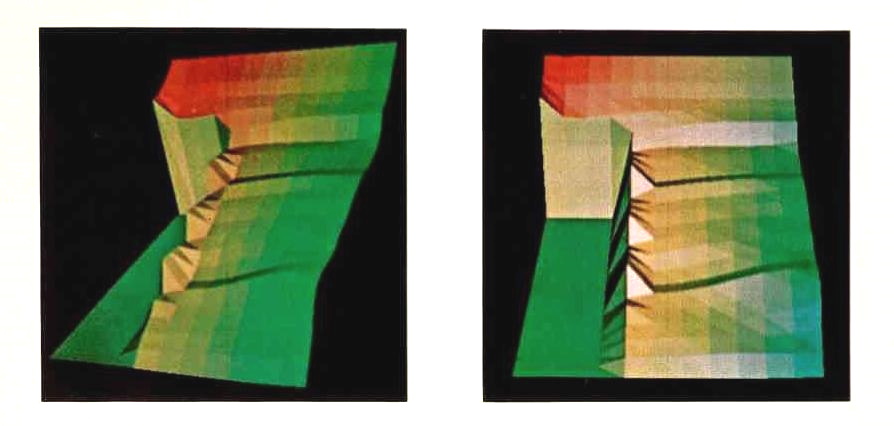
These two figures represent different views of a two-dimensional surface in four-dimensional space. Here variation in hue on the surface represents variation in the fourth variable. Red indicates high values and green indicates low values. Orange, yellow, and yellow-green indicate intermediate values.
1. Appel, A, Some Techniques for Shading Machine Renderings of Solids, SJCC68, Pp. 37-45.
2. Evans, Ralph M, et al, Principles of Color Photography, New York: 1953, Wiley.
3. Floyd, Robert W, ' Nondeterministic Algorithms, JACM, XIV, No. 4 (October, 1967), pp. 636-644.
4. Roberts, L G, Homogeneous Matrix Representation and Manipulation of N-Dimensional Constructs, Notes for English Summer Conference Course, University of Michigan, 1965.
5. Sutherland, I E, Computer Graphics-Ten Unsolved Problems, DATAMATION, XII, No. 5 (May, 1966), Pp. 22-27.
6. Warnock, John E, A Hidden Line Algorithm for Halftone Picture Representation, Technical Report 4-5, Salt Lake City, Utah, University of Utah, 1968.
7. Weiss, R A, BE VISION, A Package of IBM 7090 FORTRAN Program to Draw Orthographic Views of Plane and Quadric Surfaces, JACM, XIII, No. 2 (February, 1966), pp. 194-204.
8. Wylie, C, et al, Half-Tone Perspective Drawings by Computer, FJCC67, (1967), Pp. 49-58.