Half-tone perspective drawings by computer

Chris Wylie, Gordon Romney, David Evans, Alan Erdahl

University of Utah

FJCC 1967

1. INTRODUCTION

In recent years, the sheer increase in demand for the graphic presentation of three-dimensional objects has almost overhwelmed conventional facilities; that is, designers, draftsmen and especially engineering artists. For example, it is important for a designer or architect to quickly describe a three-dimensional object and view it immediately; not as an endless set of engineering drawings, but as if he were viewing the three-dimensional object itself. He should be able to take a distant look at a complicated object, and then view, in detail, any subsection of the object. In other words, he would like to quickly and cheaply simulate and view the thing he is designing.

The goal of this project is to provide a system which will display images that a person can feel, as contrasted with images that he must laboriously interpret (e.g., the engineering drawings of an airplane).

Several subjective factors apparently help the viewer's ability to feel the overall structure of a three-dimensional object: 1) binocular (or stereo) vision, 2) elimination of the hidden surfaces, 3) recognition of distance and shape as a function of illumination (or shading), and 4) real time movement.

For a display algorithm to be practical, the computing time should grow only linearly with the complexity of the object and the resolution of the display. Other workers

(Lawrence G Roberts, Lincoln Laboratory)

have found that, with their methods for the hidden surface problem, the computing time grew very rapidly with complexity. Thus, the display of significant objects was thus impractical.

There were other disadvantages. Roberts used rectangular solids and prisms to construct objects. This is a severe limitation when dealing with curved or Riemannian surfaces. To get around this difficulty, we have used triangles to describe objects. For example, it is easily seen that it is impossible to completely cover the surface of a sphere with quadrangles. However, it can be done quite conveniently with triangles (Figure 1).

Any developable surface can be approximated arbitrarily accurately with small, but finite, triangles (Figure 1). Another reason for using triangles is that three points always determine a plane. In this case many results from geometry and linear algebra have attractive forms for computation.

Figure 1 - Example of one method of approximating a sphere by planar triangles

The object, and its perspective projection on a view plane, are examined by a scanning ray extending from a view point (Figure 2).

Figure 2 - Perspective projection of triangles onto the view plane

2. OVERVIEW OF THE ALGORITHM

2.1 Background Concepts

2.1.1 Basic geometry of the problem

Everything is ultimately referred to an underlying, orthonormal vector basis E1, (Figure 3). The object is viewed from an arbitrary vantage point specified by P. The viewing plane is parallel to vectors e1, and e2. The angular orientation of the viewer about the e3 axis is determined by e1, and e2. Every three-dimensional triangle determines a two-dimensional perspective image on the view plane. In Figure 2, triangles II and III are in front of triangle I.

2.1.2. Illumination of the object

The present algorithm allows only a point source of illumination at the view point (like a single flashbulb photograph). As a consequence, there will be no shadows in the picture. The apparent brightness of a point on a surface depends on the following:

  1. The basic physical laws governing incident light, e.g., light flux varies as the inverse square of the distance from a point source, and the amount of light incident on a surface is a function of the angle of incidence (the angle between the incident ray and the normal to the surface).
  2. The nature of the reflecting surfaces, e.g., the reflectivity, texture and color may vary. We have arbitrarily chosen an inverse fourth law for computational simplicity. The user, however, may employ any relationship he desires, by modifying the appropriate subroutine.

2.1.3 Hidden surfaces problem

By far the major obstacle is solving the hidden surface problem and the means of preventing the computing time from growing faster than the number of triangles. Most of this paper will be devoted to this problem.

In solving the hidden surface problem, one could compare all the components of the entire surface for each point in the picture. This leads to a computation which likely grows at least as the product of the resolution and the number of surface elements. Instead, by using special sorting algorithms, only those triangles intersected by the scanning ray (Figure 2) need be compared.

2.2. Algorithm

This is a greatly simplified version to avoid getting bogged down in programming details.

2.2.1 Introduction

We have already assumed that any object may be approximated by a set of triangles. The input data is a set of arbitrarily ordered triangles specified by the three-dimensional coordinates of their vertices (Figure 3).

Figure 3 - Basic geometrical convention for the algorithm. The unit normal to a triangle is N. The coordinate variables are (x1,x2,x3) for the underlying basis E1 and (x1,x2,x3) for the view basis e1.

The following must be specified (Figure 3):

  1. View point, P.
  2. View basis e1.
  3. Distance from the view point to the view plane.
Figure 4 - Illustration of the ratio |R|/r being equal to R3/r3

2.2.2 Per frame calculation

The view plane is examined by a systematic scanning raster (Figure 5). One complete raster scan of the view plane will be called a frame (One side benefit of the raster scan is the inherent compatibility of the method with television-type display devices).

Figure 5 - Slice made by the sweep of a scanning ray
  1. Preprocess the triangles: The algorithm begins with the calculation of various quantities about each triangle that will be needed for later computations. They are not, however, essential in order to understand the basic method.
    1. Find the normal N, to each object triangle. This is needed in the apparent brightness calculation (Figure 3). From Figure 3, it is seen that the unit normal N, to the three-space triangle may be calculated by normalizing the vector cross product of any two of the triangle's sides.
    2. Find the apparent brightness at each object triangle's vertices, assuming the source of illumination is at the view point.
      (1) To find these brightnesses, the distances from the view (or illumination) point to each of the three vertices of the triangle must be determined. It is assumed that we have either been given (or have transformed) the components of all three-space position vectors so they are relative to the view basis.
      (2)The magnitude of a position vector to a vertex is:
      |R| = sqrt( (R1)2 + (R2)2 + (R3) 2 ) Given the unit normal of each triangle and the distance to each vertice, the user may calculate the apparent illumination of the triangle vertices with any formula he desires. The formula chosen will generally vary primarily with the nature of the reflective surface.
    3. Calculate the linear brightness interpolation parameters as in Section 2.2.5.
      Essentially, we have assumed that the apparent brightness in the interior of the view plane image of a triangle is adequately approximated by linear interpolation of the brightnesses at the three vertices of the triangle. The formula is easily derivable and will not be discussed here.
    4. Calculate the linear distance ratio parameters:
      (1) The distance ratio w along any particular scan ray is defined to be:
      w=(Distance from view point to object) / (Distance from view point to image).
      In Figure 3, w=|R| /|r| for the scan ray R to the uppermost vertex. The distance ratio is calculated for all three vertices of each triangle. For a given view point, three linear distance ratio parameters, a,b, and c, are then computed (These are recomputed when and only when the view point and orientation are changed) for each triangle such that distance ratio w, is: w=ax+by+c for any scanning ray intersecting a given triangle at view plane coordinates x and y.
      (2) The calculation of a, b, and c is based upon the fact that the distance ratio w, as defined above, is also given by:
      w = [e3 component of vector to object] / [e3 component of vector to image]
      = R3 / r3.

      The component r3, to the image, is simply the distance from the view point to the view plane, which is constant throughout a frame calculation (Figure 4).
      The component R3, to the object, is found directly from the equation of the plane which is determined by the three vertices of the three-space triangle. Note that the view plane coordinates (x,y), are effectively the same as (x1,x2), defined by the view point basis (e1 e2 e3). Because the view plane is two-dimensional and the view basis three-dimensional, there is no direct correspondence of the x3 coordinate to any view plane coordinate. The equation of the plane coincident with the three-space triangle is:
      x3 = fx1 + gx2 + h
      where f, g, and h are constants describing the plane of the object triangle and x1 and x2 are equivalent to the view plane coordinates x and y, of its image.
      Now the distance ratio is expressible in terms of the position of the scanning ray on the view plane. This is from the fact that from the projective properties of the situation (Figure 4), the distance ratio w is
      (This sort actually switches the vertex data in core storage) :
      w= |R| / |r| = R3 / r3
      Components R3 and r3 have been determined in the discussion above.
  2. Project all three-dimensional triangles onto the view plane to make a set of two-dimensional triangles (Figure 2 and Figure 3).
  3. Because the projected image is going to be scanned from top to bottom, a line at a time, all the triangles are sorted with respect to y to eliminate from consideration those triangles not crossed by the current scan line. (Figure 6).
    1. Sort the three vertices of each triangle with respect to y. (In programming this algorithm, it should be noted that various combinations of triangles present cases that require arithmetic of great precision: e.g., triangles with common edges or vertices; triangles that are coplanar, or very nearly so. These cases are not discussed here, but should be carefully examined by the programmer. From our experience, we have concluded that the description of the object and all computation should be done in integer arithmetic. Also there should be a total avoidance of division to eliminate roundoff error that would make the logic of special cases ambiguous. )
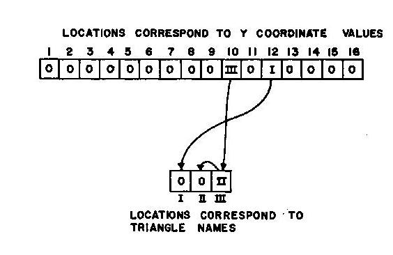
    2. The y-entrance table (Figure 7), tells which triangles are entered (i.e., begin to be intersected) by the scan line at a given y.
    3. The y-exit table, which is identical in structure to Figure 7, tells which triangles are exited by the scan line at a given y.
    4. This way we will only have to look at those triangles that a given scan line actually crosses. This avoids examining all the triangles in the entire picture at each scan line (Figure 6).
  4. Start the y-scan Every time the scan is incremented by y, the y-occupied table (Figure 8) is updated, if necessary, by looking at the y-entry and exit tables to see if a triangle has been entered or exited. In Figure 6, the scan line moves downward and triangles are entered and exited. We turn on an occupied flag when a triangle is entered and turn it off when it is exited. Each triangle has its own location in which to put an occupied flag (Figure 8). This is the first major reduction in computation.
Figure 6 - Scan line intersections of projected triangles on a simplified view plane
Figure 7 - The y-entry tables corresponding to the triangles in Figure 6. This is essentially a pointer sort indicating which triangles enter at a given y
Figure 8 - For a given y scan an occupied table indicates those triangles the scan line intersects. This figure shows a sequence of occupied tables for the entire segment of the view plane illustrated in Figure 6. Only a single row of the occupied table will exist at any instant for the current y

2.2.3 Per scan line computations

  1. For the current scan line:
    1. We go to the y-occupied table and get only the triangles that this scan line crosses.
    2. Find the x values of the intersections of the scan line with the sides of the view plane images of the triangles pulled out of the y-occupied table (Figure 6 and Figure 9).
  2. Sort each triangle's x-entry and exit intercepts into the x-entry and exit tables respectively. The x tables and sorts are identical to those used in the y-entry and exit sorts shown in Figure 7. They will not be shown in a figure.
  3. Commence moving the scan ray along the scan line by x increments.

2.2.4 Per point calculations

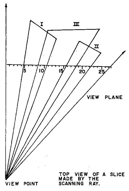
Figure 9 - Top view of a slice made by the scanning ray
Figure 10 - The visible table contains the triangle number visible at the designated x position of the scan ray
  1. For the current x, look at the x-entry and exit tables to see if there is an intersection at this x. When an intersection point is encountered, we want to know if there is a change in the visible (or hidden) status of a triangle.
    1. If there is an intersection
      1) Update the x-occupied table. The only time a triangle can change its visible or hidden status is at an intersection of the scan line and a triangle side (Figure 9).
      (We assume that no triangles cross through any other triangles. Intersecting triangles may be resolved into non-intersecting triangles by a separate algorithm prior to execution of the present half-tone perspective algorithm. )
      All these intersections are calculated for for the current scan line and are used, via manipulation of the x-entry and exit tables, to update the x-occupied table.
      (The x-occupied table has the same structure and is built in the same way as the y-occupied table. Consequently it will not be shown.)
      It is at this stage that a triangle is either added or deleted from the x-occupied table.
      2) Then go into the hidden parts calculation. (2.2.4,2)
    2. If there is no intersection, increment x and test for an intersection at the new x (i.e. increment x and go to 2.2.4,1).
  2. Hidden parts calculation
    1. Examine all triangles in the x-occupied table for the current x.
    2. Using the distance ratio parameters (computed previously in the per frame calculations Section 2.2.2, d), calculate the distance along the scan ray from the view point to each of the three-space triangles entered in the x-occupied table (Figure 9).
    3. Sort the distances to find the smallest. The triangle with the smallest distance ratio is the visible one and must be added to the visible table.
  3. Add to the visible table
    1. Figure 10 shows a completed visible table for a scan line.
    2. The contents of the table are triangle names (or numbers) showing which triangle is visible at a given x.
    3. For each x increment of the scan ray update the x-occupied table. Using the x-occupied table and the distance computation, the visible table is modified by placing the name of the visible triangle in the location corresponding to the present x value (Figure 10).
    4. The visible table is constructed for an entire scan line and is then used to find which triangle's intensity interpolation parameters are to be used for each x.

2.2.5 Per point intensity calculations

Calculate the intensities for each x in the current scan line.

  1. We interpolate to find the intensity over the visible interior of a triangle using only the intensity values at the three vertices. This allows a considerable reduction in computing time. For simplicity and speed, but not necessity, we chose linear interpolation. The linear interpolation parameters have already been calculated and stored during the per frame calculations (Section 2.2.2, c).
  2. The formula for the intensity at a point x on the scan line y is I=ax+by+c where I is the intensity and a, b, c are the linear interpolation parameters for the visible triangle.

2.2.6 Output to display device

The list of intensities for this scan line is sent to a peripheral device for eventual display. The output subroutines are distinct and independent of the half-tone algorithm to permit flexibility as the display hardware is improved or altered.

3. RESULTS

3.1 Program

A FORTRAN IV program of the algorithm (Figure 11), called PIXURE has been written (Modifications of this program and some new work are progressing rapidly) and used to produce half-tone pictures of a cube and tetrahedron (Figures 13 through 18). For both the cube (12 triangles) and the tetrahedron (4 triangles) the execution time of PIXURE was roughly 25 seconds to calculate a frame of 512 × 512 points on a Univac 1108. PIXURE at present is approximately 3800 Univac 1108 assembly language instructions in length and occupies 14K 36-bit words of storage for a picture of 100 triangle complexity.

Preliminary tests indicate that the execution time is most dependent on the number of scan lines that intersect the two-space image of the object (e.g. there are eleven scan lines, 2 ≤ y ≤ 12, that intersect triangles in Figure 6). It also appears that this dependence is very closely linear. On the other hand, execution-time dependence on the number of triangles (i.e. the number of intersection points per scan line) appears to be much better than linear. The dependence on the number of hidden traingles per intersection point has not been rigorously determined but seems to be close to linear.

Figure 11 - Flow chart of the half-tone perspective algorithm

3.2 Hardware techniques

Each scan line that PIXURE generates is sent to a PDP-8 via a specially designed interface (Figure 12). The PDP-8 serves essentially as 1) a buffer, 2) a raster generating device for an oscilloscope, and 3) an a-synchronous I/O channel communicating with the 1108. Each scan line, in turn, is stored in the PDP-8 memory and then transmitted through a digital to analog (D-A) converter to a Tektronix 453 oscilloscope. The scan position is dictated by ten bit x and y registers in the D-A converter. The intensity of the beam at each point in the scan is controlled by a six bit z register. Due to storage and 108 PDP-8 transmission-rate limitations we have been forced to take time exposure photographs of the scope trace. As soon as a scan line is completed, the PDP-8 requests information for the next scan line. For a 512 × 512 frame it takes approximately ten seconds to generate a picture.

Figure 12 - Display system

3.3 Subjective interpretations

The principal objective of this project is to allow people to see three-dimensional objects, as realistically as possible, using two-dimensional images (or displays). We have chosen to erase hidden surfaces and use half-tone shading to give the illusion of depth (or distance) and indicate spatial relationships. Although we are presently limited to a single source of illumination at the view point; nonetheless, the pictures of our test objects show obvious dimensionality.

Figures 13, 14 and 15 represent a cube whose resolution differs by a factor of ten. It is evident that Figure 14, representing a picture of 512 × 512 points, supplies sufficient information to adequately describe the cube. A more critical test on the resolution of the receding edge could not have been made, and yet, the edge appears tn the higher resolution pictures. The unusual perspective, however, was merely the result of an arbitrary choice in geometry. The apparent triangular composition of the cube faces has since been corrected and a smooth transition across triangle boundaries achieved (Figure 16).

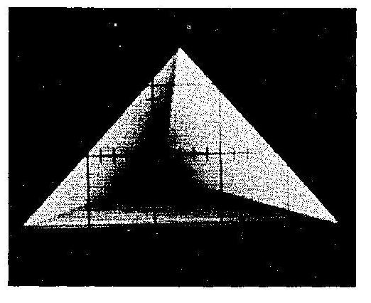
The pictures of the tetrahedron (Figure 17 and Figure 18) are superior in quality to those of the cube for two reasons. First, a defect in the display hardware was partially corrected, resulting in a more even display pattern. Scan lines are still noticeable, but it is felt that additional improvement in the hardware will significantly diminish this defect. The second improve- ment was in the selection of a more correct range of intensity levels used in the brightness calculation.

Another objective is to display an object so that it will not be ambiguously interpreted. The tetrahedron in Figure 17 is decidedly convex, but Figure 18 could be either convex or concave unless the source of illumination be specified.

Figure 13 - Cube 100 × 100
Figure 14 - Cube 512 × 512
Figure 15 - Cube 1024 × 1024
Figure 16 - Cube 512 × 1512
Figure 17 - Tetrahedron 512 × 512
Figure 18 - Concave tetrahedron 512 × 512 (one side removed)

SUMMARY

In the cases we have tested, the computing time grows almost linearly with the resolution of the picture, the size of the visible portion of the object and apparently, the amount of hidden surface. This makes the algorithm practical, and is a result of special sorting techniques which greatly reduce the number of hidden surface comparisons required. The objects we have displayed appear quite three-dimensional and their hidden surfaces are effectively eliminated. The computing time required for a picture composed of over 106 points was approximately 40 seconds on a Univac 1108.

The present system definitely proves the feasibility of the real-time display of two-dimensional half-tone images. It is felt that the technique may be easily extended to stereo representation of half-tone images. Furthermore, the algorithm is so constructed as to allow computations to be executed in parallel (see the dotted section in Figure 11). As many scan lines as hardware permits may be calculated simultaneously. Also, much of the computation may be performed by incremental hardware. The parallel and incremental characteristics of the algorithm lead us to believe that real-time movement and display of half-tone images is very near realization.

A typical user wishes to describe an object in a form convenient for him. Also, a flexible and extensive data structure must be constructed to contain and manipulate an object. Therefore, the practical application of the algorithm depends greatly on the ability of the system to convert an object into a suitable mesh of triangles. Our group has initiated work in these directions and at present has a triangle generation algorithm operational for objects composed of planar surfaces.

ACKNOWLEDGMENTS

The authors are deeply indebted for the programming assistance of Lee Copeland and Richard Blackburn. The technical skills of Richard Jepperson, Charles Eder and Y. T. Kim have assisted immensely in helping produce the first photographs. And, last but not least, we wish to thank the University of Utah Computer Center for their patience and assistance in making these results possible.

BIBLIOGRAPHY

A L FASS and A R AMIR-MOEZ, Elements of linear spaces, Macmillan Company New York 1962

B E MESERVE, Fundamental concepts of geometry Addison-Wesley Reading Mass I 955

L G ROBERTS, Homogenous matrix representation of N-dimensional solids, MIT Lincoln Laboratory Lexington Mass

L G ROBERTS, Machine perception of three-dimensional solids, MIT Lincoln Laboratory 1963 Technical Report no 315 Lexington Mass

More Computer Animation Papers 1964-1976