
Simulating physical phenomena by finite difference (or finite element) computer programs places many burdens on the user. Foremost among these are verification of input data and interpretation of output results. In 3D programs the problems become acute, since it is difficult to convey 3D information on conventional 2D media, especially as numbers. (If a 2D dump is an array, with rows being one dimension and columns the other, where do we put the third dimension?) Hence, graphical display is a prime necessity in running and understanding 3D codes. VPIX 3D provides the user with many of the required capabilities in the graphics area.
VPIX 3D generates pictures of 3D objects in proper perspective with all hidden lines removed. The program is interactively capable of rotating, translating, and scaling the object in the field of view. VPIX 3D sends its pictures to a variety of output devices, including teletypewriter (TTY), dd80, television monitor display system (TMDS), dd80A, and indirectly, grey-level TMDS. It displays 3D meshes, either as line drawings or half-tone pictures shaded from a light source, and can be used to display input mesh to check their validity, or the coordinates of node points output by the main program to display distortions caused by displacement. The program also generates pictures with shading done according to some problem variable (e.g., temperature) and pictures with surface contours determined, as in the shading, by an arbitrary variable.
The subroutines that perform the perspective calculation, hidden line removal, and packing of data required by the various output media were written by Mike Archuleta of the LLL Computer Graphics Group. In particular, the subroutines that remove hidden lines (no mean task} are an implementation of the Watkins' algorithm for the LLL 7600 network (OCTOPUS). Their rapid performance makes feasible the semi-interactivity of the program.
The program operates from TTY, with the user supplying commands that indicate how he wishes to look at the object, and where he wants the picture to go. It expects as input a data file (on disk) with the following characteristics in order: a 512 word header, all x coordinates, all y coordinates, all z coordinates, and finally all variable values. (Note that the variable values need not be present in the file if the user simply wishes to display the mesh geometry.) In graphical form, the file looks like this:
| Header |
|---|
| x |
| y |
| z |
| Variable (e.g. temp.) |
The header contains the following data:
| WORD (abs. disk. addr. | Information |
|---|---|
| 0 | Number of "blocks" in the file> |
| 1 | Total number of node points for all blocks together. |
| 2-11 | Total number of node points for each block individually. |
| 12-21 | Number of node points per plane for each block. |
| 22-31 | Number of planes per block (IPT). |
| 32-41 | Number of points in j-direction for each block (JPT). |
| 42-51 | Number of points in k-direction for each block (JPT). |
| 52-512 | Available for future use. |
(Note that there are a maximum of ten blocks in a problem and that the x-y-z data starts at absolute disk address 10008).
An explanation is in order. VPIX 3D was written primarily as a service routine for the finite difference code, HEMP 3D, and the finite element code, SAP. The meshes for these problems are very regular in the sense that they are composed of eight-node "bricks" arranged in a regular fashion or "block." A block is typified as consisting of a number of planes (taken in one of the three logical directions, i, j, or k), with the number of node points being constant in each plane. An object may consist of several blocks. Figure 1 presents a simple two-block problem and the header associated with it.
One might question what this type of organization buys the user. To see any advantage, one must first look at the hidden-line subroutines. These routines operate on polygons; clipping, sorting, storing them, etc. In this application, the polygons are simply the rectangular faces of the zones. Now, since our blocks are very regular, the algorithm used to pick the coordinates of these polygons (zones) out of the data file is relatively simple. What's more, we can easily pick out and pass to the hidden-line subroutines only those polygons on the surface. This simplifies their work and implies the possibility of displaying larger objects (i.e., the interior zones of the mesh are already known to be hidden; the fact needn't be discovered by the hidden-line algorithm).
The data in the file is defined in a standard three-dimensional "right-handed" Cartesian coordinate system. Since the hidden surface algorithm perversely uses a left-handed system, the program will transform the data to present the picture correctly. In manipulating the picture, however, the user must employ the left-handed system. Essentially, the eye is at the origin looking "down" the positive z-axis (into the screen) with positive y being up and positive x to the right. The field of vision is limited to a pyramid defined by the planes, z = ±x, and z =±y, Figure 2.
The initial view is a picture of the bottom of the object. It is up to the user to alter this view, if he so desires.
Usually no single picture reveals everything one wishes to know about a particular object. Therefore the program enables the user to rotate the object around its center point, move the object up or down, left or right, or toward or away from him, and to scale the object (zoom in or out). There is also a "slicing" option, allowing him to look at the interior of the object. The commands are input from the teletype and may be "'stacked" (i.e., more than one command per TTY line).
-----------------------------------------------------------------------

     LOCATION (CEC.)             CONTENTS

-----------------------------------------------------------------------
         0                       1   ------ NUMBER OF BLOCKS '
         1                     378   ------ TOTAL POINTS ALL BLOCKS
         2                     324   ------ POINTS IN BLOCK 1
         3                      54   ------ POINTS IN BLOCK 2
       4 THROUGH 11              0
        12                      81   ------ POINTS PER J-K PLANE BLOCK 1
        13                       9   ------ POINTS PER J-K PLANE BLOCK 2
      14 THROUGH 21              0
        22                       4   ------ IPT BLOCK 1
        23                       6   ------ IPT BLOCK 2
      24 THROUGH 31              0   ------
        32                       9   ------ JPT BLOCK 1
        33                       3   ------ JPT BLOCK 2
      34 THROUGH 41              0
        42                       9   ------ KPT BLOCK 1
        43                       3   ------ KPT BLOCK 2
        44 THROUGH 49            0
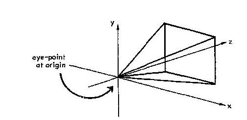
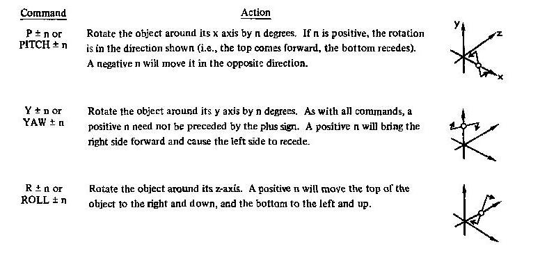
Figure 3 depicts the results of commands that enable the user to revolve the object about its center point. The center point is located on the z-axis of the viewing system. It is sometimes helpful to imagine a separate "object coordinate system" associated with this point. The rotations can then be thought of as changing this system in relation to the coordinate system of the viewer. The user should practice with these commands until he is familiar with them, and must remember that they are not commutative. (A YAW 45, then PITCH 45, is not always the same view as a PITCH 45, then YAW 45.)
The translation commands are very simple to understand. They move the object along axes. Where the rotation commands enable one to see all sides of an object, the translation commands will move the object around in the field of view.


There is a single command that holds the object in place and makes it larger or smaller. This enables the user to concentrate on details of greatest interest to him.
Command                  Action
S n or SCALE n           Multiplies the coordinates of the picture
                         by n while holding the center point fixed.
                         (Note: the command will accept a negative
                         n but this has the same effect as
                         YAW 180 SCALE n.)
The first part of the hidden line algorithm removes all lines that lie outside the viewing "window" or screen, a process known as "clipping." Ordinarily, the routine clips to the planes establishing the viewing pyramid (ie,z=±x,±y). However, it can also clip to two other z-planes (Z = ZMAX, ZMIN) and thus remove even more of the picture. If the limits of the object being viewed are beyond the two planes in either, or both, directions ie., OBIMAX ≥ ZMAX, OBJMIN ≤ ZMIN), then part of the object is removed. Thus, one can "slice" through an object and examine its interior. Figure 4 depicts a cube being sliced progressively along a diagonal.
However, this introduces a problem; i.e., the interior must be present before it can be examined. If you will remember, the program usually passes only the exterior coordinates to the hidden-line subroutines, since it "knows" all interior points are hidden anyway. Now, since the user can slice the object arbitrarily, the program no longer knows which interior points are "automatically" hidden. Therefore it chooses the coward's way out; it passes the coordinates of all the polygons to the hidden line algorithm, and asks it to decide which are hidden.

The user should be well aware of the extra burden he is placing on the routine in doing a slice. There is a limit to the number of polygons the hidden-line subroutines can handle and, if the user chooses too large a slice. they will run out of space and send an error message. The option is then to choose a smaller slice, or quit.
          Command                                Action
User: SLICE                      The routine will go into "slicing mode" and
Routine: ZMAX= ZMIN=             inform the user of the present ZMAX and ZMIN.
          TYPE NEW ZMAX ZMIN     It will then ask the user for a new ZMAX and
User:  n n                       ZMIN. The user then specifies the limits of
                                 the slice. and the routine will go about its
                                 business.

         NOSL                    Turn off the slicing option. Should be turned
                                 off, whenever it is unneeded, for efficient
                                 operation.
In analyzing the output of 3D problems, it is often desirable to examine the value of certain problem variables at various locations on, or in the problem mesh. One method of doing this is to display lines of constant value, contours, on the problem grid. Figure 3 and Figure 4 are examples of such plots. The contour plotting commands in VPIX 3D allow the user to specify the number of contour levels he wishes to calculate and to select among any of those levels for any single picture.
          Command                                Action

CONTR n                          Turn on the contour option and set up n contour
                                 levels. This sets up an array, CLEVEL. with n
                                 entries (n ≤  39). Where
                                 CLEVEL(1) = VMIN + (((VMAX-VMIN)/(n-1))*(I-1))

HILO nhi nlo                     Resets two internal variables, CONHI and CONLO.
                                 Initially, CONHI = VMAX and CONLO = VMIN.

                                 The program will plot contours for an values of
                                 CLEVEL between CONHI and CONLO.

                                 Thus, one can selectively delete or add contours
                                 by the use of this command. (NOTE: VMAX and VMIN
                                 are the maximum and minimum value of the problem
                                 variable associated with 1he grid, and are
                                 typed-out for you by VPIX 3D.)

NOCON                            Turn off the contour plotting option. (It is
                                 initially turned off.)
VPIX 3D produces two types of smooth-shaded half-tone pictures. In the first type, shading is done according to a light source located at infinity behind the user (i.e., a planar source). In the other, shading is done much like the contour plotting: i.e., the light intensity is assigned according to the variable value. Those grid points associated with the highest values receive the greatest intensities (appear brightest).
          Command                                Action
LITE                             Do shading according to a light source (This is the
                                 initial mode)

VARS                             Do shading according to the associated problem variable.
Added versatility is obtained by permitting the object to be broken down into smaller components. These exploded views can add to the understanding of complex geometrics by focusing attention on a specific area. Increased visibility can be attained by changing the scale in a given direction compared to the other two directions. Also, it is possible to remove the grid lines and show only the outside profile of the object. This is useful where contour plots are to be superimposed on the surfaces of the object. Examples appear in Figure 5.
VPIX 3D will output its pictures io a variety of media. The user must specify the output medium each time in order to produce a picture.
          Command                                Action
TV n                               Sends picture to TMDS monitor n. The picture will
(TV)                               appear in the form of a line drawing. Once you
                                   get a monitor, just type TV, or the program gets
                                   confused.

DD80                               Sends the picture to dd80 file. The file is kept
                                   by the user and has the name, VPICa, where "a" is
                                   some arbitrary letter. This file can be "given
                                   away" using ALLOUT. The first call to this will
                                   cause the program to request box and ID information.

DD80A                              Does nothing now, since the dd80A is not on-line.
                                   Will produce hardcopy of greyscale and color
                                   pictures.

GREY or                            Sends a shaded picture to a disk file (program
G32                                asks for name). GREY produces shaded pictures
                                   with 8 levels of intensity; G32 gives 32 levels.
                                   The pictures can subsequently be viewed on the
                                   grey-level TMDS monitor by using Archuleta's
                                   GREY controller.

TTY                                Sends picture to your teletypewriter. The picture
                                   will be a block of numbers showing the shading
                                   with "0" being the background intensity, and "9"
                                   being the highest intensity. This will give the
                                   user a rough idea of the shading.
          Command                                Action

NEXT                               Closes the old data file and asks the user to
                                   specify a new one.

RSND                               Cause the picture to be resent to the most
                                   recently specified medium without reprocessing
                                   picture. For use after TMDS error.

END                                Disengages program control and goes away nicely.

A number or features will be included in VPIX 3D in the future. These include the possibilities for generating color pictures on the dd80A and also for generating movies. The former will come when the dd80A comes on-line and the latter when need arises.
To run VPIX 3D you need the controllee and a data file. To initialize, type:
VPIX3D I t V or VPIX3D filename / t v
The filename is the name of the input data file. If one is at specified on the execute line, the program will ask for one. lf the grid has a problem variable associated with it, the first message will be
VMAX = n VMIN = n
After that, whenever the program is ready to receive commands, it will type the prompt "OK." Commands are blank delimited and may be stacked (e.g. P90 Y 180 TV 68 DD80). Numbers may be input as integers or as floating points. If you misspell any command, leave out a blank, or omit a numeric argument that should be there; you will get an error message, and any commands left in the stack will be ignored.